The Straightest Tool in the Shed

The First Regression in the World

In 1885, Francis Galton was studying the height of parents and their children. He noticed something curious, tall parents tended to have tall children, but those children were usually a little shorter than their parents. Short parents had short children, but slightly taller ones. Everything seemed to drift back toward the average.

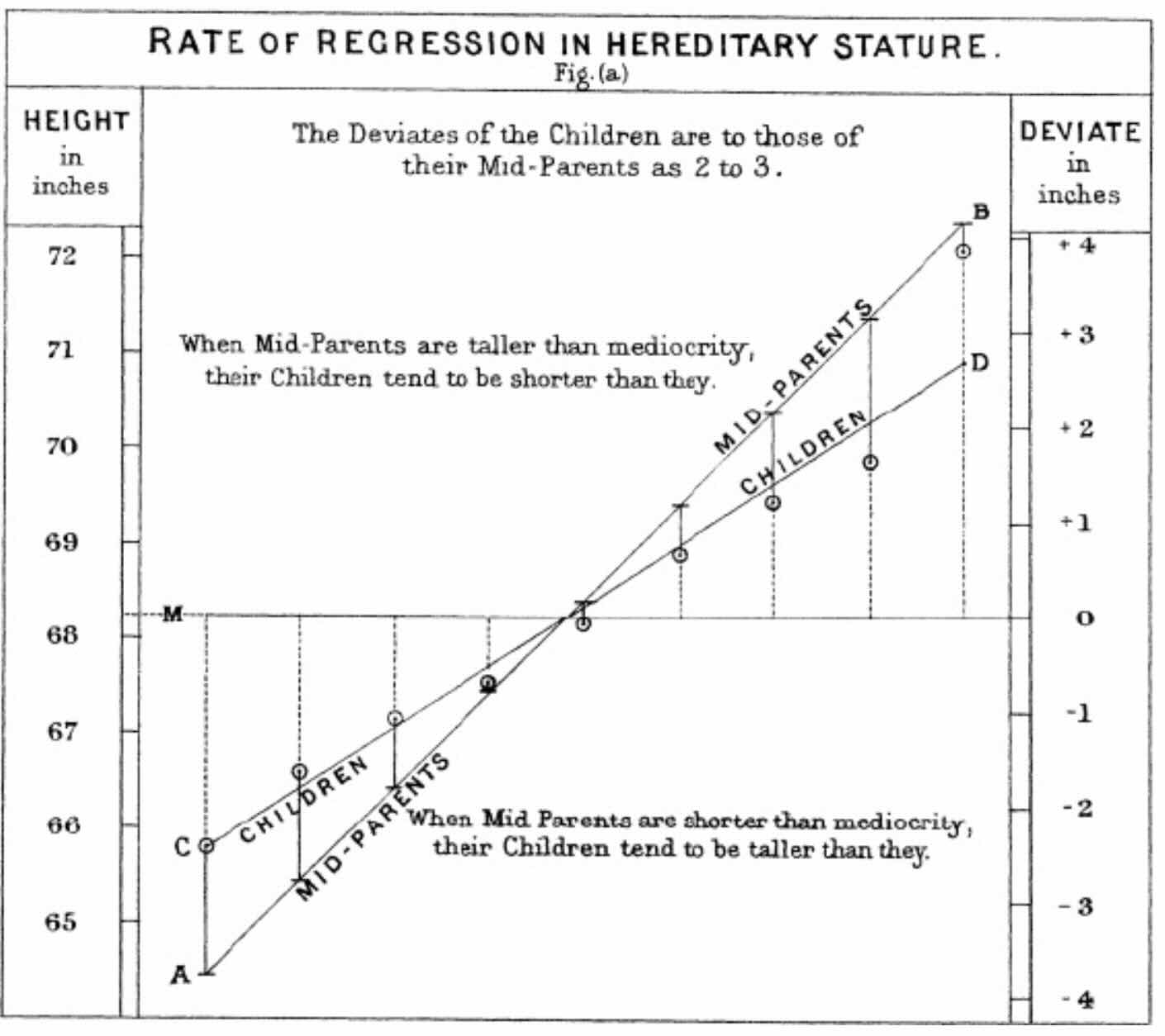
Rate of regression in hereditary stature (Galton 1886 Plate IX, fig. a)

He called this phenomenon "regression to the mean", and the name stuck, long after the concept grew into something far more powerful.

What Galton was really doing, without modern language for it, was drawing a line through a cloud of points. A line that best captured the relationship between two things: parent height and child height. That line is what we now call a regression line, and the method he used to find it inherited the name. We still call it regression today.

What is linear regression?

At its heart, linear regression is finding the best straight line through a set of data points. Given two variables, say, hours studied and exam score, or house size and price, we want to describe how one changes as the other changes. That line has a simple form:

$$\hat{y} = w_0 + w_1 \, x$$

$x$ is what we know (the input, e.g. hours studied)
$\hat{y}$ is what we predict (the output, e.g. exam score)
$w_1$ is the slope, how much $\hat{y}$ changes when $x$ increases by 1
$w_0$ is the intercept, where the line crosses the vertical axis when $x = 0$

The challenge: how do we find the best values of $w_0$ and $w_1$?

In $\hat{y} = w_0 + w_1 x$, which parameter controls how steeply the line rises?

The Analytical Solution, Finding the Best Line

"Best" needs a definition. The most natural one: the best line is the one that minimizes the total prediction error between predictions and actual data points. We call these differences residuals.

To avoid positive and negative errors cancelling each other out, we square them and take the average. This gives us the Mean Squared Error (MSE):

$$L(w_0, w_1) = \frac{1}{n}\sum_{i=1}^{n}\bigl(y_i - w_0 - w_1 x_i\bigr)^2$$

The beautiful thing about this problem is that it has an exact, closed-form solution. Using calculus, we set the derivatives of $L$ with respect to $w_0$ and $w_1$ to zero and solve. The result is:

$$w_1 = \frac{\displaystyle\sum_{i=1}^{n}(x_i - \bar{x})(y_i - \bar{y})}{\displaystyle\sum_{i=1}^{n}(x_i - \bar{x})^2}$$

$$w_0 = \bar{y} - w_1 \bar{x}$$

Where $\bar{x}$ and $\bar{y}$ are simply the averages of $x$ and $y$. The numerator of $w_1$ measures how $x$ and $y$ move together; the denominator measures how much $x$ varies on its own.

In matrix form, useful when we have many input variables, this becomes even more compact:

$$\mathbf{w} = (X^\top X)^{-1} X^\top \mathbf{y}$$

Plug in your data, compute the formula, and you immediately get the optimal line. No guessing, no iteration, just math.

Does finding the optimal weights for linear regression require an iterative algorithm?

Regression as Machine Learning, Teaching a Line to Learn

Now let's shift perspective. What if, instead of solving the formula directly, we taught a computer to find the best line through trial and error? This is where linear regression becomes the simplest example of a machine learning algorithm.

The setup has five ingredients:

Data We have a dataset: pairs of inputs $x_i$ and outputs $y_i$. This is what the model will learn from.
A model with parameters Our model is the line $\hat{y} = w_0 + w_1 x$. The weights $w_0$ and $w_1$ are knobs we can turn. At first, we set them randomly.
A loss function We need a way to measure how bad our current line is. There are multiple losses out there that we will discuss in the course. Here let us use the Mean Squared Error (MSE):
$$L(w_0, w_1) = \frac{1}{n}\sum_{i=1}^{n}(y_i - w_0 - w_1 x_i)^2$$
The larger this value, the worse our line fits the data. Our goal: make it as small as possible.
Gradient descent, walking downhill Imagine the loss function as a hilly landscape. You are standing somewhere on that landscape, and you want to reach the lowest valley. The strategy: look around, find the direction that goes downhill the fastest, and take a small step that way. Repeat.
That "downhill direction" is given by the gradient, the partial derivatives of $L$:

$$\frac{\partial L}{\partial w_1} = -\frac{2}{n}\sum_{i=1}^{n} x_i(y_i - w_0 - w_1 x_i)$$

$$\frac{\partial L}{\partial w_0} = -\frac{2}{n}\sum_{i=1}^{n}(y_i - w_0 - w_1 x_i)$$

At each step, we update the weights by moving against the gradient (since we want to go downhill):

$$w_1 \;\leftarrow\; w_1 - \alpha \cdot \frac{\partial L}{\partial w_1}$$

$$w_0 \;\leftarrow\; w_0 - \alpha \cdot \frac{\partial L}{\partial w_0}$$

Where $\alpha$ (alpha) is the learning rate, the size of each step. Too large, and you overshoot the valley. Too small, and it takes forever to get there.
A stopping criterion We need to know when to stop. Common choices: run for a fixed number of iterations, or halt when the loss stops decreasing meaningfully. Without a stopping rule, gradient descent would run forever, getting marginally better with each step but never quite finishing.

What does the learning rate $\alpha$ control in gradient descent?

Now Try It Yourself

You and a partner each get your own weight space, a 2D plane of possible $(w_0, w_1)$ pairs. Click anywhere in your panel to test that combination. Dots glow red when you are close to a good fit and blue when you are far. After each guess you'll see Warmer or Colder compared to your own previous attempt. Ten turns total, alternating. Lowest MSE wins.

Why Does This Matter?

For linear regression, gradient descent is overkill, we have the exact formula. But the real power is that this same loop:

data → model → loss → gradient descent → stopping criterion

…is the engine behind every neural network, every large language model, every modern AI system. The architecture changes. The loss function changes. The gradients get more complex. But the loop stays the same. Linear regression is where that story begins.

Tinker with the Code

The game is written in Python using Pygame, so you can open main.py and modify it directly. Try changing the number of turns, the range of weights, or the amount of noise in the dataset, even small tweaks can reveal a lot about how the loss landscape behaves. The source code is available here:

https://github.com/i-yam/passt/tree/main/modules/hot_or_cold